A Short Introduction to Quantum Optimal Control

2025-07-17

This handout was written to accompany a talk I gave during the Institute for Pure and Applied Mathematics' long workshop on non-commutative optimal transport. You can download the original PDF handout, or read the HTML version below.

Abstract

We first give a short definition of quantum states and operators, and explain how quantum states evolve in time. We then explain what quantum optimal control is and how to frame it as a nonlinear programming (optimization) problem which can be solved computationally. Finally, we explain the GRAPE technique. Some simplifications have been made to keep this accessible –- for example, real hardware implementations of qubits are often infinite-level systems, but we treat them here as two-level systems.

Quantum Computing

The state of a closed quantum system can be represented by a complex-valued state vector $\boldsymbol{\psi} \in \mathbb{C}^N$. Each observable [A quantity that can be physically measured.] of the system is associated with a Hermitian matrix $O \in \mathbb{C}^{N \times N}$. The eigenvalues of the operator are the possible outcomes of the measurement [Because the matrix is Hermitian, the eigenvalues are real, which makes sense because the eigenvalues are physically measurable quantities.] , and the corresponding eigenvectors are the states for which that measurement will be observed. We may write the state vector in terms of the orthonormal eigenvectors of $O$:

Then $|c_i|^2$ gives the probability of observing the state $\boldsymbol{\psi}_i$ when the system is measured, upon which the system is said to collapse to the measured state. For this reason, the coefficients $\{c_i\}$ are called probability amplitudes. Consequently, the length of the state vector is $\| \boldsymbol{\psi} \|_2^2 = 1$ at all times because the probabilities of observing each possible outcome must sum to one. This also implies that the time evolution of the state vector is unitary, since unitary matrices preserve length.

In the quantum computing literature, states are often represented using bra-ket notation, where we may denote a state by $|\psi\rangle$. The state $\boldsymbol{\psi} \in \mathbb{C}^N$ represents $|\psi\rangle$ in a particular measurement basis. Similarly, a matrix $O$ represents the operator $\hat{O}$ in a particular basis. In other words, $|\psi\rangle$ is just a way of labeling a physical state, whereas a corresponding state vector $\boldsymbol{\psi} \in \mathbb{C}^N$ gives information on the outcomes of measuring the system. We switch between the two notations when convenient, but mostly stick to representing states as complex-valued vectors. [$|\boldsymbol{\psi}\rangle$ is called a ket, and $\langle\boldsymbol{\psi}| \sim \boldsymbol{\psi}^\dagger$ is called a bra. Cutely, the bracket $\langle\psi_\alpha|\psi_\beta\rangle = \boldsymbol{\psi}_\alpha^\dagger \boldsymbol{\psi}_\beta$ represents an inner product. Many by-hand calculations can be simplified using inner products and orthonormality of eigenvectors, so this notation can be convenient when working with pen and paper.]

In this work, we only consider closed quantum systems. In a quantum computing context, this means considering only time scales short enough that there is no significant interaction between the quantum computer and the environment. Open quantum systems, which model the interaction between the quantum computer and the environment, are much larger and more computationally challenging, but the algorithms for performing quantum optimal control on them are essentially the same as for closed quantum systems.

Governing Equation: Schrödinger's Equation

The time evolution of the state vector from an initial state $\boldsymbol{\psi}_0$ in a closed quantum system is governed by Schrödinger's equation [We always choose our units so that $\hbar=1$.]

where $H(t) \in \mathbb{C}^{N \times N}$ is the Hamiltonian of the system, the matrix corresponding [In the sense of observables, described in the previous section.] to the measurement of the total energy of a system. [Schrödinger's equation is a postulate of quantum mechanics. It cannot be derived, but the idea that the dynamics of a quantum system are determined by the linear operator corresponding to the energy of the system can be classically motivated; in Hamiltonian mechanics, the dynamics of a classical system are determined by the Hamiltonian function of the system, which usually gives the total energy of the system.]

In most quantum computing hardware, the Hamiltonian takes the form:

$H_d$ is called the drift Hamiltonian, because even when the functions $f_1,\dots,f_{N_c}$ are all zero, the state vector still drifts because of the dynamics caused by $H_d$. [The term system Hamiltonian is also used to describe $H_d$.] $H_{c,1},\dots,H_{c,N_c}$ are called the control Hamiltonians, because in a quantum computer the control functions $f_1,\dots,f_{N_c}$ correspond to the amplitude of laser pulses (or something similar) which we can program in order to control the dynamics of the system.

Defining the Quantum Optimal Control Problem

Quantum optimal control refers to the process of manipulating the Hamiltonian in (1, 2) to implement some desired behavior. The two most common types of quantum optimal control problems are state transfer problems and gate design problems.

State Preparation Problems

In a state preparation problem, we start from some known quantum state $\boldsymbol{\psi}_0$ which can easily be prepared on a quantum computer. [Usually, the initial state is the ground state of the quantum computer, which the quantum computer naturally relaxes to over time.] We want to transfer the state to some desired state $\boldsymbol{\psi}_{\textrm{Target}}$ over some period of time $0 \leq t \leq T$. Because the Hamiltonian controls the dynamics of the system, we do this by searching for a Hamiltonian which causes the desired dynamics.

In order to quantify the "closeness" of two quantum states, we use the fidelity between the two states:

The fidelity has several properties which make it a good way to quantify the "closeness" of two quantum states.

1. The fidelity between two states $F(\psi_\alpha, \psi_\beta)$ is $1$ when $\psi_\alpha = \psi_\beta$, and $0$ when the two states are orthogonal.

2. The fidelity does not depend on the global phase of the states. That is, $F(e^{i\delta_\alpha}\boldsymbol{\psi}_\alpha, e^{i\delta_\beta}\boldsymbol{\psi}_\beta) = F(\boldsymbol{\psi}_\alpha, \boldsymbol{\psi}_\beta)$ for all $\delta_\alpha, \delta_\beta \in \mathbb{R}$. This is physically significant because the global phase of a state cannot be measured. [This means that the states $\sqrt{2}^{-1}(\boldsymbol{\psi}_0+\boldsymbol{\psi}_1)$ and $e^{i\delta}\sqrt{2}^{-1}(\boldsymbol{\psi}_0+\boldsymbol{\psi}_1)$ are indistinguishable. However, we can measure a relative phase, so the states $\sqrt{2}^{-1}(\boldsymbol{\psi}_0+\boldsymbol{\psi}_1)$ and $\sqrt{2}^{-1}(\boldsymbol{\psi}_0+e^{i\delta}\boldsymbol{\psi}_1)$are distinguishable, although their probability amplitudes have the same magnitude.]

Then we can write our optimal control problem as

We are trying to find control functions $\{f_i\}$ which implement a Hamiltonian which minimizes the infidelity between the initial state and the target state.

I have no idea how to solve this optimization problem computationally, since I have no idea how to program a computer to search over the spaces of arbitrary functions $f: \mathbb{R} \rightarrow \mathbb{R}$. [If you know how to do this, please let me know!] And analytic solutions are only known for a select few problems that involve very small quantum systems. To solve the optimization problem computationally, we introduce the control vector $\boldsymbol{\theta} \in \mathbb{R}^{n_c \cdot N_c}$ to parameterize the control functions. Each control function is a linear combination [In principle, the dependence may be nonlinear, but using a linear dependence keeps the parameterization of the control functions simple. A linear dependence is also computationally useful because it makes taking the gradient of the control functions trivial.] of $n_c$ basis functions. [In principle, the number of basis functions can be different for each control function, but keeping the number the same makes it easier to write.] For notational convenience, we can write the control vector in matrix form as $\Theta \in \mathbb{R}^{n_c \cdot N_c}$, with $\Theta_{j,k} = \boldsymbol{\theta}_{(j-1)n_c + k}$.

The choice of the basis functions $\{b_{j,k}\}$ is called the control pulse ansatz.

We can finally write our optimization problem as

[The semicolon in $f(t;\boldsymbol{\theta})$ just indicates that $\boldsymbol{\theta}$ does not change often like $t$ does. We optimize over $\boldsymbol{\theta}$, but we only ever solve Schrödinger's equation for a constant value of $\boldsymbol{\theta}$.] We are searching for control parameters $\boldsymbol{\theta}$ which determine the control functions $\{f_i(t;\boldsymbol{\theta})\}$, which determine the Hamiltonian $H(t)$, which controls the dynamics of the system, in order to minimize the infidelity between $\boldsymbol{\psi}(T)$ and the target state $\boldsymbol{\psi}_{\textrm{Target}}$.

Written in terms of $\boldsymbol{\theta}$, the optimization problem is now a nonlinear programming (NLP) problem with no constraints, where Schrödinger's equation is solved numerically to find $\boldsymbol{\psi}(T)$ and evaluate the objective function in (5). Constraints may be added, for example to keep the amplitude of the control functions below some maximum determined by experimental constraints. This NLP may be solved by direct-search methods [E.g. Nelder-Mead.] , or by gradient-based methods. [E.g., gradient descent, ADAM, or quasi-Newton methods such as L-BFGS.] True second-order Newton methods could also be used, but they require computing the Hessian of the objective function, which is very computationally expensive.

Gate Design Problems

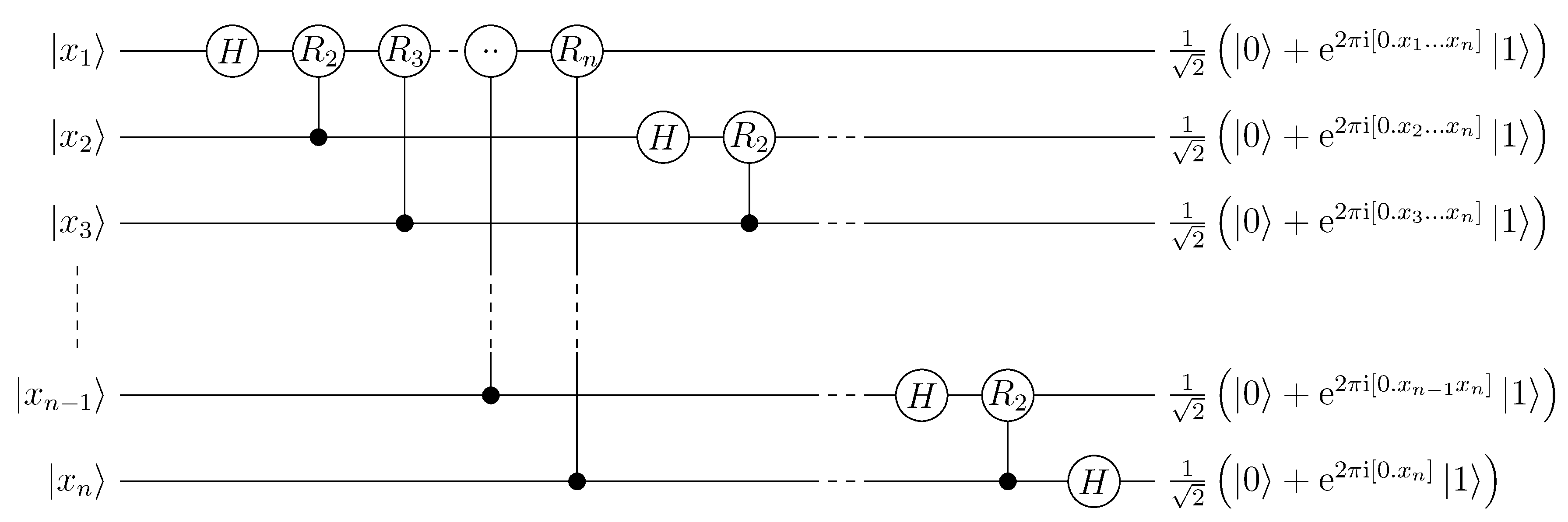
Quantum gates are the basic building blocks of quantum algorithms. In this way, they are analogous to classical logic gates. [AND, OR, NOT, XOR, etc.] Each gate is a unitary transformation which acts on a subsystem of the full quantum system. [E.g., it operates on only a few qubits in a quantum computer consisting of many qubits.] An algorithm may be specified using a circuit diagram, which maps out the gates used in a quantum algorithm, which qubits they are applied to, and in what order.

To characterize a gate, it is sufficient to know how the gate transforms the elements of a basis of the subsystem. This allows us to specify a gate using a truth table, the same way we would specify a classical logic gate. For example, the truth table of a CNOT (Controlled NOT) gate is given below, and the matrix representation of the gate (i.e. the unitary transformation it applies, in the standard/computational basis) follows.

Roughly speaking, this is very similar to the state preparation problem, only now we are looking for a Hamiltonian which transfers several initial states to several corresponding target states. Strictly speaking, we are looking for a Hamiltonian which generates a target unitary matrix $U_{\textrm{Target}}$. To see why optimizing for a specific target unitary matrix is different than optimizing the ability of the unitary to prepare several final states from several initial states, consider the unitaries $U_A = \left[\begin{smallmatrix} 0 & 1 \\ 1 & 0 \end{smallmatrix}\right]$ and $U_B = \left[\begin{smallmatrix} 0 & 1 \\ i & 0 \end{smallmatrix}\right]$. We have $U_A |0\rangle = |1\rangle$, $U_A|1\rangle=|0\rangle$, $U_B|0\rangle=i|1\rangle$, $U_B|1\rangle=|0\rangle$. Because the global phase of a state cannot be measured, from a multiple state preparation point of view, the two unitaries both "perfectly" perform the state preparations $|0\rangle \rightarrow |1\rangle$, $|1\rangle \rightarrow |0\rangle$. The unitaries create different relative phases (which are measurable) when they operate on states other than the initial states in the state preparation problems: $U_A\sqrt{2}^{-1}\left(|0\rangle+|1\rangle\right)=\sqrt{2}^{-1}\left(|1\rangle+|0\rangle\right)$, $U_B\sqrt{2}^{-1}\left(|0\rangle+|1\rangle\right)=\sqrt{2}^{-1}\left(i|1\rangle+|0\rangle\right)$.

When we say a Hamiltonian generates a unitary matrix, we mean that the dynamics caused by the Hamiltonian (according to Schrödinger's equation) can be represented by a unitary time-evolution matrix $U(t)$:

We want to choose a Hamiltonian (parameterized through $\boldsymbol{\theta}$), which over a period of time $0 \leq t \leq T$ generates a unitary $U(T)$ that is "close" to $U_{\textrm{Target}} \in \mathbb{C}^{N \times N}$. As before, we need a way to quantify the "closeness" of two unitaries. We use the gate infidelity:

[The Frobenius inner product $\langle A, B \rangle_F = \operatorname{Tr}[A^\dagger B]$ can be computed simply as $\sum_{j,k} \overline{A}_{j,k}B_{j,k}$.] As with the state fidelity, the gate infidelity takes a value between $0$ and $1$, and is invariant to changes in the global phase of the unitaries.

Just as we did with state preparation problems, we parameterize the control functions in terms of a control vector $\boldsymbol{\theta}$ so we can formulate the quantum optimal control problem as an NLP problem, which can be solved computationally. [$I_N$ denotes the $N$ by $N$ identity matrix.]

GRAPE Optimization

Optimizing even a two-qubit state transfer or gate design problem is moderately challenging, and three-qubit problems are quite difficult. [Especially when the qubits are not treated as true two-level systems, but as 3 or 4 level systems, which is more accurate (technically, for most quantum computing architectures each qubit has an infinite number of levels).] As the systems become more difficult to control, more control parameters are typically needed in order to find a suitable set of control functions. The increased number of control parameters make the optimization more challenging due to the increased number of search dimensions, but gradient-based methods excel at navigating high-dimensional optimization landscapes. [Although as the number of qubits increases, many optimization tasks suffer from the barren plateau problem, which makes optimization extremely difficult even with gradient-based methods.] To use these methods, we need to be able to compute the gradient. A naive way is to approximate the partial derivatives of the objective function using finite differences, e.g.

[We denote the $n$-th vector in the standard basis by $\boldsymbol{e}_n$.] but then the gradient is inexact, and most importantly, computing the gradient a single time requires solving at least as many Schrödinger equations as there are control parameters.

The GRAPE (GRadient Ascent Pulse Engineering) method (Khaneja et al., 2005) cleverly computes the gradient exactly, and with a cost of solving only two Schrödinger equations, regardless of the number of control parameters. It does this by using a piecewise constant control pulse ansatz, where the gate duration is divided into $n_c$ time intervals of width $\Delta t = T/n_c$, and the control functions are constant during each time interval. Specifically, in (4), the basis functions are

Simply stated, $\Theta_{j,k}$ is the amplitude of the $j$-th control function during the $k$-th time interval. [This control pulse ansatz may seem arbitrary, but the control functions are usually shaped using arbitrary waveform generators, for which the idealized output is piecewise constant.]

For simplicity, we will consider a problem with only one control Hamiltonian, and no drift Hamiltonian.

Because the Hamiltonian is constant across each time interval, the time evolution across each interval can be computed using matrix exponentials. And we can write the time evolution across the whole duration as

Now, the partial derivatives of the gate infidelity are

Performing the matrix multiplications and evaluating the traces in the above expression is cheap, but computing $\partial U(T) / \partial \theta_n$ [$\partial U(T) / \partial \theta_n$ is sometimes called a sensitivity.] for each $n=1,\dots,n_c$ is expensive. Naively, they could be obtained for each $\theta_n$ by solving a system of ODEs [Perhaps we could have suspected this intuitively. Changing a control parameter changes the dynamics, so to know how the state at the end of the dynamics changes with respect to each control parameter we need to look at a new dynamical system for each control parameter.] similar to Schrödinger's equation, but with a forcing term. [This is actually done in the GOAT (Gradient Optimization of Analytic ConTrols) method (Machnes et al., 2018).]

But, because only the $n$-th unitary in (8) depends on $\theta_n$, we can write $\partial U(T)/\partial \theta_n$ analytically as the simple expression

Evaluating the partial derivative only involves inserting one extra matrix multiplication into the sequence of unitaries that we apply to $U(0)$ in order to get $U(T)$. Even better, we can write

and

Then the procedure is to first compute $U(T) = U_{n_c} \cdots U_1 U(0)$. Then, for $n = n_c,\dots,1$, use (10) to compute $U_{\textrm{Target}}^\dagger (\partial U(T)/\partial\theta_n)$. Because $U_{n+2}^\dagger\cdots U_{n_c}^\dagger U_{\textrm{Target}}$ and $U_{n-1}\cdots U_1 U(0)$ were already computed during the previous iteration, this only requires computing two matrix exponentials [The matrix exponentials $U_1,\dots,U_n$ may be computed once and stored, if there is sufficient memory available.] and performing three matrix-matrix multiplications, which is much less expensive than computing $n_c$ matrix exponentials [Computing matrix exponentials is a computationally expensive operation, which is a drawback of the GRAPE method.] and performing $n_c+1$ matrix-matrix multiplications, which is the cost of computing and multiplying all the unitaries in (10). During each iteration, once we have computed $U_{\textrm{Target}}^\dagger (\partial U(T)/\partial\theta_n)$, we can use (9) to compute the $n$-th partial derivative of the objective function (the infidelity). This concludes the method.

The GRAPE method was an important development, made around 2005. Since then, major improvements have been made, but modern developments in open-loop [In quantum optimal control, open-loop means completely simulation-based, with no experimental feedback. If there is experimental feedback, the method is called a closed-loop method.] quantum optimal control generally still rest on doing some kind of forward evolution, adjoint evolution scheme which produces exact gradients and does not scale heavily in cost with the number of control parameters.

The GRAFS (GRadient Ascent in Function Space) method (Lucarelli, 2018) uses a similar technique as the GRAPE method; the control functions are piecewise constant, and the time evolution is performed using matrix exponentiation, which allows the gradient to be computed analytically and cheaply (using a forward solve and an adjoint solve). The major difference is that although the control pulses are piecewise constant, the control parameters do not correspond directly to the amplitudes of the control functions across each time interval. Instead, the control functions are parameterized in terms of continuous basis functions, as we did in (4). The control functions are then discretized into piecewise constant functions, and the relationship between the control parameters and the discretized function amplitudes is used to compute the gradient in an efficient way, similar to the GRAPE method.

Questions

I have some questions I can't answer because I don't know enough about classical optimal control theory. I would appreciate any input from people more familiar with classical optimal control!

1. What would the Hamilton-Jacobi-Bellman equations look like for a quantum optimal control problem, and why don't we solve the quantum optimal control problem by solving the Hamilton–Jacobi–Bellman equations? [My guess is that it has to do with the curse of dimensionality.]

2. Are the GRAPE method and similar methods (methods that use a forward/adjoint scheme to compute the gradient) the same as Pontryagin's maximum principle? If not, why don't we use it? [According to section 3 of the GRAFS paper (Lucarelli, 2018), GRAPE is essentially Pontryagin's maximum principle with trivial costate dynamics.]